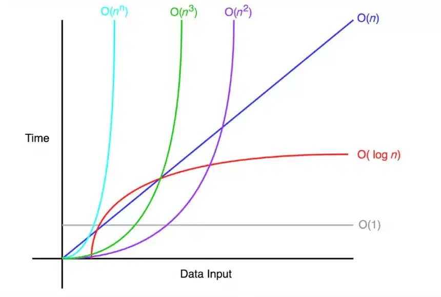
Big-O notation
In this tutorial, we are going to discuss about the Big-O notation. Big-O notation is a mathematical notation that is used to describe the performance or complexity of an algorithm, specifically how long an algorithm takes to run as the input size grows.
Understanding Big-O notation is essential for software engineers, as it allows them to analyze and compare the efficiency of different algorithms and make informed decisions about which one to use in a given situation. In this tutorial, we will cover the basics of Big-O notation and how to use it to analyze the performance of algorithms.
What is Big-O?
Big-O notation is a way of expressing the time (or space) complexity of an algorithm. It provides a rough estimate of how long an algorithm takes to run (or how much memory it uses), based on the size of the input. For example, an algorithm with a time complexity O(n) of means that the running time increases linearly with the size of the input.
What is time complexity?
Time complexity is a measure of how long an algorithm takes to run, based on the size of the input. It is expressed using Big-O notation, which provides a rough estimate of the running time. An algorithm with a lower time complexity will generally be faster than an algorithm with a higher time complexity.
What is space complexity?
Space complexity is a measure of how much memory an algorithm requires, based on the size of the input. Like time complexity, it is expressed using Big-O notation. An algorithm with a lower space complexity will generally require less memory than an algorithm with a higher space complexity.
Examples of time complexity
Here are some examples of how different time complexities are expressed using Big-O notation:
O(1): Constant time. The running time is independent of the size of the input.O(n)O(n²)O(logn)O(2n)

Big-O notation uses mathematical notation to describe the upper bound of an algorithm’s running time. It provides a way to compare the running time of different algorithms, regardless of the specific hardware or implementation being used.
It’s important to note that Big-O notation only provides an upper bound on the running time of an algorithm. This means that an algorithm with a time complexity of O(n) could potentially run faster than an algorithm with a time complexity of O(logn) in some cases, depending on the specific implementation and hardware being used.
Additionally, Big-O notation only considers the dominant term in the running time equation. For example, an algorithm with a running time of O(n²+n) would be simplified to .

Example algorithms and their time complexities
1. Linear search - O(n)
O(n)Here are a few examples of algorithms along with their time complexities expressed using Big-O notation:
package com.ashok.datastructures.linearsearch;
/**
 *
 * @author ashok.mariyala
 *
 */
public class LinearSearch {
    public static int linearSearch(int[] arr, int x) {
        for (int i = 0; i < arr.length; i++) {
            if (arr[i] == x) {
                return i;
            }
        }
        return -1;
    }

    public static void main(String[] args) {
        int[] arr = {3, 5, 7, 9, 11};
        int x = 7;
        System.out.println(linearSearch(arr, x));
    }
}
This linear search algorithm has a time complexity of O(n)n, the linear search will take n steps to complete.
2. Binary search - O(logn)
O(logn)package com.ashok.datastructures.binarysearch;
/**
*
* @author ashok.mariyala
*
*/
public class BinarySearch {
public static int binarySearch(int[] arr, int x) {
int low = 0;
int high = arr.length - 1;
while (low <= high) {
int mid = (low + high) / 2;
if (arr[mid] < x) {
low = mid + 1;
} else if (arr[mid] > x) {
high = mid - 1;
} else {
return mid;
}
}
return -1;
}
public static void main(String[] args) {
int[] arr = {2, 3, 4, 10, 40};
int x = 10;
System.out.println(binarySearch(arr, x));
}
}This binary search algorithm has a time complexity of O(logn)n, it will take approximately log(n) steps to complete the binary search.
3. Bubble sort – O(n²)
O(n²)package com.ashok.datastructures.bubblesort;
/**
*
* @author ashok.mariyala
*
*/
public class BubbleSort {
public static void bubbleSort(int[] arr) {
int n = arr.length;
for (int i = 0; i < n; i++) {
for (int j = 0; j < n - i - 1; j++) {
if (arr[j] > arr[j + 1]) {
int temp = arr[j];
arr[j] = arr[j + 1];
arr[j + 1] = temp;
}
}
}
}
public static void main(String[] args) {
int[] arr = {64, 34, 25, 12, 22, 11, 90};
bubbleSort(arr);
for (int i : arr) {
System.out.print(i + " ");
}
}
}This bubble sort algorithm has a time complexity of O(n²)
That’s all about the Big-O notation. If you have any queries or feedback, please write us email at contact@waytoeasylearn.com. Enjoy learning, Enjoy Data Structures.!!