Big-O notation
In this tutorial, we are going to discuss about the Big-O notation. Big-O notation is a mathematical notation that is used to describe the performance or complexity of an algorithm, specifically how long an algorithm takes to run as the input size grows.
Understanding Big-O notation is essential for software engineers, as it allows them to analyze and compare the efficiency of different algorithms and make informed decisions about which one to use in a given situation. In this tutorial, we will cover the basics of Big-O notation and how to use it to analyze the performance of algorithms.
What is Big-O?
Big-O notation is a way of expressing the time (or space) complexity of an algorithm. It provides a rough estimate of how long an algorithm takes to run (or how much memory it uses), based on the size of the input. For example, an algorithm with a time complexity O(n) of means that the running time increases linearly with the size of the input.
What is time complexity?
Time complexity is a measure of how long an algorithm takes to run, based on the size of the input. It is expressed using Big-O notation, which provides a rough estimate of the running time. An algorithm with a lower time complexity will generally be faster than an algorithm with a higher time complexity.
What is space complexity?
Space complexity is a measure of how much memory an algorithm requires, based on the size of the input. Like time complexity, it is expressed using Big-O notation. An algorithm with a lower space complexity will generally require less memory than an algorithm with a higher space complexity.
Examples of time complexity
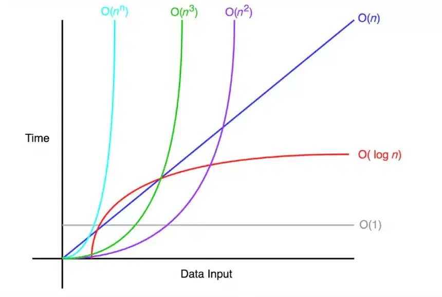
Here are some examples of how different time complexities are expressed using Big-O notation:
O(1): Constant time. The running time is independent of the size of the input.O(n)O(n²)O(logn)O(2n)
Big-O notation uses mathematical notation to describe the upper bound of an algorithm’s running time. It provides a way to compare the running time of different algorithms, regardless of the specific hardware or implementation being used.
It’s important to note that Big-O notation only provides an upper bound on the running time of an algorithm. This means that an algorithm with a time complexity of O(n) could potentially run faster than an algorithm with a time complexity of O(logn) in some cases, depending on the specific implementation and hardware being used.
Additionally, Big-O notation only considers the dominant term in the running time equation. For example, an algorithm with a running time of O(n²+n) would be simplified to .

Example algorithms and their time complexities
1. Linear search - O(n)
Here are a few examples of algorithms along with their time complexities expressed using Big-O notation:
package com.ashok.datastructures.linearsearch;
/**
 *
 * @author ashok.mariyala
 *
 */
public class LinearSearch {
    public static int linearSearch(int[] arr, int x) {
        for (int i = 0; i < arr.length; i++) {
            if (arr[i] == x) {
                return i;
            }
        }
        return -1;
    }

    public static void main(String[] args) {
        int[] arr = {3, 5, 7, 9, 11};
        int x = 7;
        System.out.println(linearSearch(arr, x));
    }
}
This linear search algorithm has a time complexity of O(n)n, the linear search will take n steps to complete.
2. Binary search - O(logn)
package com.ashok.datastructures.binarysearch;
/**
 *
 * @author ashok.mariyala
 *
 */
public class BinarySearch {
    public static int binarySearch(int[] arr, int x) {
        int low = 0;
        int high = arr.length - 1;
        while (low <= high) {
            int mid = (low + high) / 2;
            if (arr[mid] < x) {
                low = mid + 1;
            } else if (arr[mid] > x) {
                high = mid - 1;
            } else {
                return mid;
            }
        }
        return -1;
    }

    public static void main(String[] args) {
        int[] arr = {2, 3, 4, 10, 40};
        int x = 10;
        System.out.println(binarySearch(arr, x));
    }
}
This binary search algorithm has a time complexity of O(logn)n, it will take approximately log(n) steps to complete the binary search.
3. Bubble sort – O(n²)
package com.ashok.datastructures.bubblesort;
/**
 *
 * @author ashok.mariyala
 *
 */
public class BubbleSort {
    public static void bubbleSort(int[] arr) {
        int n = arr.length;
        for (int i = 0; i < n; i++) {
            for (int j = 0; j < n - i - 1; j++) {
                if (arr[j] > arr[j + 1]) {
                    int temp = arr[j];
                    arr[j] = arr[j + 1];
                    arr[j + 1] = temp;
                }
            }
        }
    }

    public static void main(String[] args) {
        int[] arr = {64, 34, 25, 12, 22, 11, 90};
        bubbleSort(arr);
        for (int i : arr) {
            System.out.print(i + " ");
        }
    }
}
This bubble sort algorithm has a time complexity of O(n²)
4. Quick Sort - O(n * logn)
package com.ashok.datastructures.quicksort;

import java.util.ArrayList;
import java.util.List;

/**
 *
 * @author ashok.mariyala
 *
 */
public class Solution {
    public static List<Integer> quickSort(List<Integer> arr) {
        if (arr.size() <= 1) {
            return arr;
        }
        int pivot = arr.get(arr.size() / 2);
        List<Integer> left = new ArrayList<>();
        List<Integer> middle = new ArrayList<>();
        List<Integer> right = new ArrayList<>();
        for (int x : arr) {
            if (x < pivot) left.add(x);
            else if (x > pivot) right.add(x);
            else middle.add(x);
        }
        List<Integer> sorted = new ArrayList<>();
        sorted.addAll(quickSort(left));
        sorted.addAll(middle);
        sorted.addAll(quickSort(right));
        return sorted;
    }

    public static void main(String[] args) {
        List<Integer> arr = List.of(3, 6, 8, 10, 1, 2, 1);
        List<Integer> sortedArr = quickSort(arr);
        System.out.println("Sorted array: " + sortedArr);
    }
}
This implementation of quick sort has a time complexity of O(n * logn), on average. In the worst case, the time complexity is O(n²), if the pivot is always the smallest or largest element in the array.
The quick sort algorithm works by selecting a pivot element and partitioning the array into three subarrays: one containing elements less than the pivot, one containing elements equal to the pivot, and one containing elements greater than the pivot. It then recursively sorts the left and right subarrays.
The time complexity of quick sort is determined by the number of recursive calls that are made. Each recursive call processes approximately elements, so the total number of recursive calls is approximately log(n). The running time of each recursive call is O(n) , so the total running time is O(n * logn).
5. Fibonacci sequence - O(2n)
Here is an implementation of an algorithm for calculating the n’th element of the Fibonacci sequence:
package com.ashok.datastructures.fibonacci;
/**
 *
 * @author ashok.mariyala
 *
 */
public class Solution {
    public static int fibonacci(int n) {
        if (n == 0) {
            return 0;
        } else if (n == 1) {
            return 1;
        } else {
            return fibonacci(n - 1) + fibonacci(n - 2);
        }
    }

    public static void main(String[] args) {
        int n = 10;  // Example input
        System.out.println("Fibonacci number at position " + n + " is " + fibonacci(n));
    }
}
This implementation of the Fibonacci sequence has a time complexity of O(2n), which is exponential in the size of the input. This is because each call to fibonacci(n) results in two additional recursive calls to fibonacci(n-1) and fibonacci(n-2).
The time complexity of this algorithm is determined by the number of recursive calls that are made. Each recursive call processes one element, so the total number of recursive calls is approximately 2n. The running time of each recursive call is O(1), so the total running time is O(2n).
That’s all about the Big-O notation. If you have any queries or feedback, please write us email at contact@waytoeasylearn.com. Enjoy learning, Enjoy Data Structures.!!